
INTRODUCTION
Hello, again! Today, I will be exploring the exciting world of Regression! I will be predicting housing prices using the Ames Housing Dataset, provided by Kaggle. I will do this by implementing a simple Linear Regression model using Python and SciKit-Learn. That being said, what exactly is Regression?
Regression (in the context of machine learning) is a supervised machine learning model that is used to predict continuous values. Examples of continuous values could be something like someone’s height or the price of a house. This is unlike classification, which predicts values that are countable and discrete. For this dataset, I will be implementing Linear Regression which is a specific type of regression model. So how does Linear Regression work?
We all learned the equation of a line in grade school… The infamous “y = mx+b“. Linear regression is essentially the process of finding a line that best fits the given data. However rather than having a single independent variable (x), it will likely have many (x1, x2, x3… xn) depending on the data, thus creating a hyper plane. Simple enough right?

So how do we determine what line fits best? This is done by measuring residuals. Given a line, a residual is the shortest distance between a point and the line. We can calculate the fit of the line by summing all the residuals squared for each data point. The smaller that number is, the better.

Once a line of best fit has been chosen, how can we determine how effective it is at fitting the data? Just because we have the best line does not necessarily imply that it actually is a useful fit.
To determine how effective our line is, there are a number of statistics we could use. However, R-squared or the coefficient of determination is probably the most popular. R-squared is the proportion of the variation of the dependent variable that is predictable from the independent variables.

R-squared essentially measures the goodness of fit of a model. A value of 1 indicates that the model perfectly predicts the data.
Another way to measure the goodness of fit is by the Root Mean Square Error (RMSE). RMSE is the standard deviation of the residuals. Intuitively, this measures how spread out the residuals are which indicates how concentrated the data is around the line of best fit.

Initial Data Inspection
Now that we have an idea of what linear regression is, we can begin to implement it. As stated before, we will be predicting the prices of houses in Ames, Iowa. Let’s go ahead and start some initial inspections of the data.

81 features! That’s a lot of data and thankfully the creator of the dataset provided a description of each feature.

After checking nulls, we can see that some columns contain many nulls. We can also already see some indications of multi-collinearity, based on the features that contain the same exact amount of nulls and related names. We’ll discuss multi-collinearity a bit further later.
Based on the provided data descriptions and initial inspection, we can see that there is quite a bit of categorical columns. Categorical columns can be a bit more involved to work with since they will not directly be compatible with a linear model.

Experiment 1
Now that we have an initial understanding of our data, we can start our first “experiment”. At this point, I’ve dropped features with more than 300 null values, temporarily removed all categorical features, filled remaining nulls with a 0 value, and dropped the ‘Id’ column since it only really represents row index.
The goal of this first experiment is really just to throw the initial data at a regression model without much pre-processing. I want to set a baseline and build from there.

So our initial model returned an R-squared score of about 0.65. Honestly, considering how minuscule pre-processing was done, and how much of the data was stripped, it is not too bad of a score.
I am curious to see how standardizing the data will effect the initial score. I imagine it should increase some since linear regression is know to benefit from scaling.
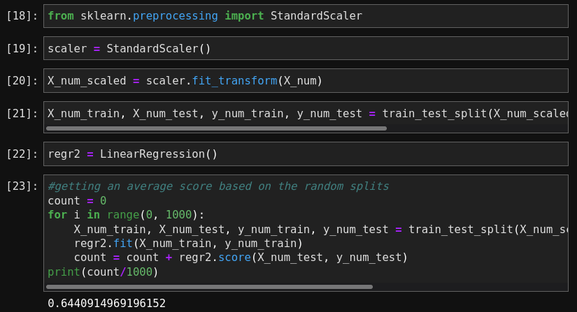
Surprisingly, the score is almost the same as before… not sure why. Next, I want to try training on more than just the continuous features. Note that before, I removed categorical variables, even ones that are numerical. Let’s see how the model performs after re-adding these features.

Looks like our score jumped 10%! Not too bad at all.
I think that pretty much covers the initial model testing. I know there is certainly plenty of room for improvement. Let’s explore what additional and more involved pre-processing is needed.
Experiment 2
For this next experiment, I will be exploring some more pre-processing options. When cleaning and processing data, I think it is very important to keep the model that you are using in mind as different models have different requirements. For linear regression there are a number of assumptions that should be accounted for.
- Linearity
- Homoscedasticity (Constant Error Variance)
- Independence of errors
- Multivariate Normality
- No or little Multi-collinearity
Having said this, let’s see if our data fits some of these assumptions.
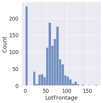


After exploring the features, many of them are relatively normal, which is good. I did notice that our dependent variable, sale price was slightly skewed. We can apply a log transformation to normalize it.
Next, let’s further explore our categorical features so see if some look like they are correlated with SalePrice.


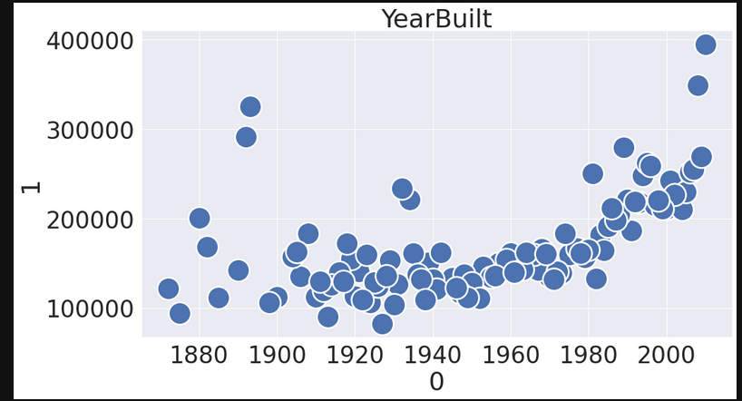
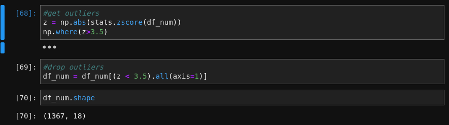
Only a handful of the features seemed to be correlated, visually at least. It was certainly apparent that outliers may be causing issues for the model as well. Let’s go ahead drop outliers based on Z-score.
Alright, next let’s explore correlations.

After exploring this correlation matrix, I’ve identified a few features that are definitely correlated with each other (multi-collinearity). I’ll also go ahead and drop the features that are not very correlated with Sale Price.

Alright! I think we’re ready to train the model.

Our score jumped quite a bit! Almost .9 for our R-squared score. It’s very cool to see how much further pre-processing can help our model.
Experiment 3
For our last experiment, I’d like to try out a slightly different linear model, a Lasso Regression model. Lasso models are pretty similar to standard linear regression with the biggest difference being that it includes an L1 penalty that has the effect of shrinking the coefficients for input variables that do not contribute much to the prediction. Knowing this, I am curious to see how the Lasso model would perform when given multi-collinear features and lots of dummy variables based from the categorical features.

After throwing almost all the features at the Lasso model it performed almost just as well as our fully cleaned linear model! That’s pretty amazing!
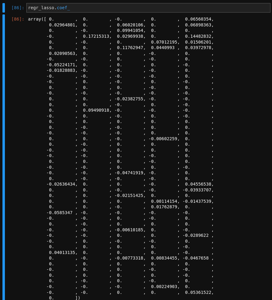
If we look at all of the coefficients of the model, we can see that it neglected a clear majority of the features!
CONCLUSION
This was definitely the largest data set I have dealt with so far in my Data Mining journey. With all that data came a lot of pre-processing! It was very clear how sensitive Linear Regression is to properly cleaned data. It was super satisfying seeing the performance improve as different cleaning techniques were performed. I loved learning about regression throughout this project and it makes me excited to keep learning about the theory of regression and different types of models. I spent a lot more time on this project than I thought I would and honestly I could of spent a lot more! There is just so much literature when it comes to regression and endless learning possibilities.
Code
The jupyter notebook for this project can be found here.
