
INTRODUCTION
As I progress in my data mining journey, learning and implementing various machine learning models will become a necessity. Of course there are different types of tasks when it comes to modeling but as the title suggests, this post will solely be focused on classification.
Classification is a form of machine learning where the predicted values are discrete. You can think of these values as bins and each prediction must fall into one of the possible bins. For instance, the data set that I will be diving into is about Iris Flowers and I will be predicting the species which is a discrete value.

That being said, the goal of this project is not necessarily to see how well I can predict the Iris species based on the data but more or less to understand the different classification models that I am using to do so. This is why I selected the Iris data set, it is tried and tested by many aspiring data scientists and is proven to be a great data set to learn from.
I will be implementing four different classification models
- Decision Trees
- K-Nearest Neighbor
- Naive Bayes
- Support Vector Machine
Each of these have their own strengths and weaknesses alike. I will be discussing them in further detail as I progress.
THE DATA
As you know, I am using the famous Iris data set. It contains four features of fifty samples of three species of Iris (Versicolor, Setosa, Virginica).
The four features are as follows
- SepalLengthCm
- SepalWidgthCm
- PetalLengthCm
- PetalWidthCm

The data set can be found here. Also, here’s a great article about the history of this famous data set.
PRE-PROCESSING AND DATA UNDERSTANDING
The Iris data was already cleaned and pretty much ready to go out of the box. Subtle processing steps were undertaken to setup each model.
I converted the species names into numerical values to ensure compatibility with the models.
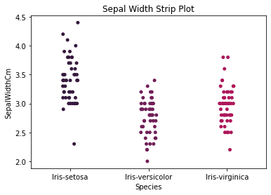
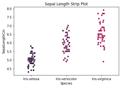
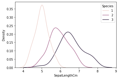
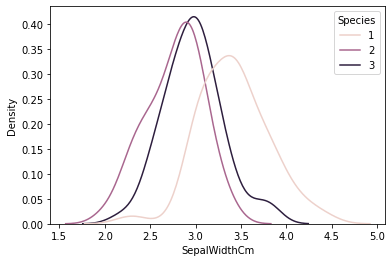
I also decided to create two other data frames; one for the petal measurements and one for the sepal measurements. I decided to do this because of the visualizations I created, it was very apparent that the sepal measurements had more overlap than the petal measurements (specifically within the Versicolor and Virginica species). So I’d like to see how the models perform when only given certain features.
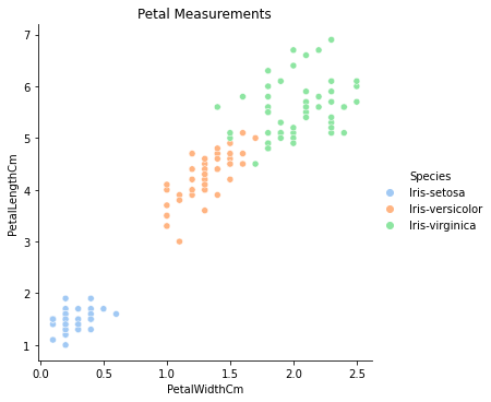
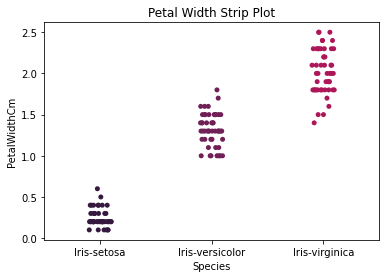
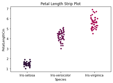
Here are some further visualizations do understand the relationship between the features and each class.
How does each species correspond with each measurement?

DATA MODELING
As stated before I will be implementing four classification algorithms. The first of which is the decision trees algorithm.
Decision Trees can be used for both regression and classification tasks. They create a decision structure in the form of a tree of nodes and edges. Decision trees are a great option if you want to be able understand exactly why the model is doing what it’s doing. This is known as a white box algorithm. Due to the nature of the tree structure, it is relatively easy to visualize which allows us to understand it.
The magic of the decision tree is the methods it uses to decide which features to use and what conditions to implement on these features. There are a number of metrics that do this. Two of the more commons metrics are Gini Impurity and Information gain (entropy). I won’t dive into the details of each but just know that they essentially are ways of measuring uncertainty that a certain condition of a feature will lead us to correct classification.
With this knowledge we can infer what features the decision tree will place more emphasis on. Looking at the scatter plot of the petal and sepal measurements, we know that petal measurements have much less overlap and the tree should favor those features when making decisions. That’s not to say that the sepal features will be ignored altogether, they still have value, especially when it comes to predicting the Setosa species.
I am using the scikit-learn library for implementing these models.
The code below shows the libraries used and the basic setup of the model.
from sklearn import tree
from sklearn.model_selection import train_test_split
from matplotlib import pyplot as plt

clf = tree.DecisionTreeClassifier()

X_train, X_test, y_train, y_test = train_test_split(X, y, test_size=0.3)

clf = clf.fit(X_train, y_train)
The default metric that the Scikit-learn Decision Tree uses is Gini Impurity and the default depth was 5. We can now visualize the model using MatPlotLib.
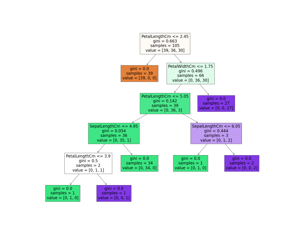
Based on the tree, we can see that the algorithm chose PetalLengthCm for its root node which is significant because it is what the algorithm thinks is the most effective for classifying the data. The tree is of depth 5 with 6 conditions considered, 4 of those conditions were petal features. It’s interesting to see that after just a single condition (the root node), the algorithm was ready to make a prediction right then and there. This really shows how distinct some the species are.
So how did our tree perform?
Our initial model produced an accuracy score of .95! Meaning it correctly classified 95% of the testing data. This is already a very good score but I’d still like to test to see if different tree depths or a different metric will make a difference.
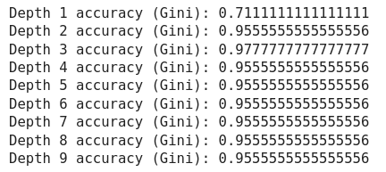

So it looks like, for our data and current model, there was no real difference between the two metrics (gini and entropy). Also it looks like the accuracy peaked at Depth 3 and had no real benefit beyond that. The f1-score for our model also resulted in .95.
Overall, our decision tree performed very well and was consistent across different parameters. This really shows how distinct the different species are and the model has no problem identifying this.
The next model that I am implementing is K-Nearest Neighbors.
K-Nearest Neighbors is another rather simple machine learning model that can be used for both regression and classification. Of course once again, I will be implementing it for classification. The algorithm operates similar to the way the name sounds. Given a new piece of data, the algorithm will classify the target based on which of the current data it is closest to (its neighbors). If you think of a traditional two dimensional graph full of random data points. When given a new point, the KNN algorithm will classify the new point based on the neighboring points that are already there.
The bulk of KNN’s computation is based on computing distance. Given this fact, it is extremely important to scale our data. Scaling our data is essentially the process of making all the data proportional with each other. Features within a data set can vary in their magnitude and units which can throw off machine learning models. Two of the more popular types of scaling are Normalization and Standardization. Normalization is the process of scaling all features so that they are between 0 and 1. Standardization on the other hand, the values are centered around the mean with a unit standard deviation.
Given how important it is to scale with an algorithm like KNN, I was curious to see how the model would perform between normalization and standardization. I am also curious about how the number of neighbors to be evaluated would effect the accuracy.
#testing different number of neighbors while standardized
for i in range(1,20):
    knn = KNeighborsClassifier(n_neighbors=i)
    knn.fit(X_train_scaled, y_train_scaled)
    print(f"(Standardized) Neighbors: {i} Score: {knn.score(X_test_scaled, y_test_scaled)}")

#testing different number of neighbors while normalized
for i in range(1,20):
    knn = KNeighborsClassifier(n_neighbors=i)
    knn.fit(X_train_n, y_train_n)
    print(f"(Normalized) Neighbors: {i} Score: {knn.score(X_test_n, y_test_n)}")
Output:

It’s interesting to see that there really is not a notable difference between the types of scaling and even the number of neighbors evaluated. Evaluating just one single neighbor produced the same score as evaluating 20… Once again I think this is just a result of how distinct our species are.
The third model I am implementing is Naive Bayes. This model is one of the most commonly implemented because of how powerful it is and considering how relatively simple it is. Naive Bayes is based off of the famous probability theorem called Bayes’ Theorem.
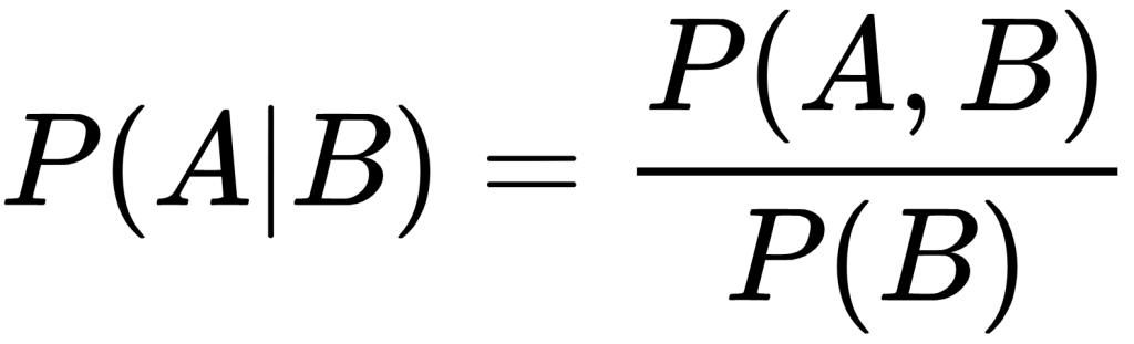
In classification or more generally, machine learning, we are are often interested in selecting the best hypothesis based on given data. Bayes’ theorem is perfect for this type of problem since it provides a way that we can calculate a probability about our hypothesis given prior knowledge about our data. This is the heart of what conditional probability is. The reason Naive Bayes is ‘naive’ is because for the sake of simpler calculations, all features are assumed to be conditionally independent. This is unlikely in real life but allows the model to be very efficient and it still performs rather well.
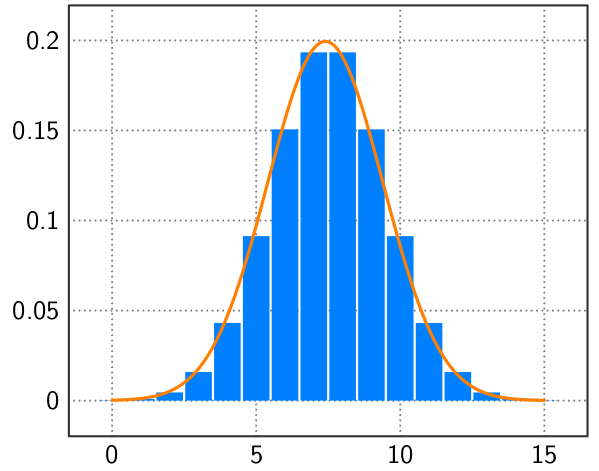
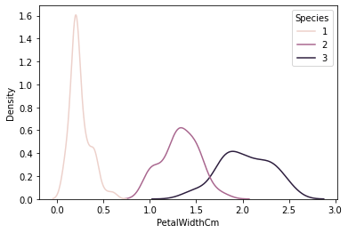
There are a number of “flavors” of Naive Bayes that can be implemented in SciKit Learn. They mainly differ in the type of distribution that is assumed of the data. In my case, I will be using Gaussian Naive Bayes since it assumes normally distributed data. I think this will be the best option since distributions of naturally occurring things such as height or weight of a person tend to be normally distributed. If we look at some density plots of our data, we can see that they look somewhat normally distributed. This is notable since our data set is rather small. As data grows, I believe that the curves would begin to smooth out more and more and become truly normally distributed.

Given this information and noting how well the other models have performed, I have high confidence in Naive Bayes
from sklearn.naive_bayes import GaussianNB

gnb = GaussianNB()
gnb.fit(X_train, y_train)

y_pred = gnb.predict(X_test)
print("Accuracy:",metrics.accuracy_score(y_test, y_pred))
As expected, Naive Bayes performed very well and produced an accuracy score of .95.
The last model I am implementing is Support Vector Machines.
The basic idea of SVM’s is pretty simple. The model tries to find a line that optimally splits the data points so that all of the data of one type of classification falls on one side of the line and data of the other type fall on the other side. However, in real life, data is almost never that well enough distinguished that a simple line could perfectly divide it. This is where kernel functions come in to play. Kernel functions manipulate all the data so that it is represented a higher dimension and then can be split by a hyper plane rather than just a line. It is such a fascinating idea to me.
Looking back at the sepal measurements plot, we can see that some of the sepal data has lots of overlap and cannot not easily be linearly separated.
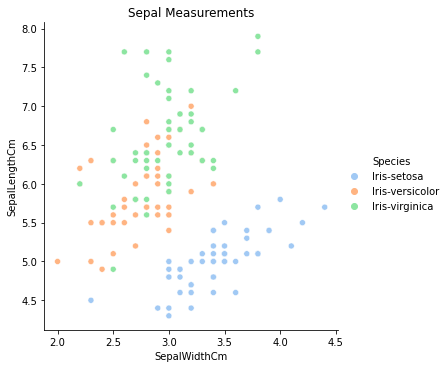
Given that, I am curious to see how a linear SVM will perform compared to a polynomial SVM when trained only on the sepal measurements.
#sepal only polynomial linear
svm_sepal_l = LinearSVC(max_iter = 5000, multi_class = 'ovr')
svm_sepal_l.fit(X_sepal_train, y_sepal_train)
svm_sepal_l.score(X_sepal_test, y_sepal_test)

#sepal only polynomial polynomial
svm_sepal = svm.SVC(kernel = 'poly')
svm_sepal.fit(X_sepal_train, y_sepal_train)
svm_sepal.score(X_sepal_test, y_sepal_test)
Well, the polynomial kernel did perform better but only slightly .8444 compared to .8222.
Also when all features are enabled, the model performed much better scoring .9777.
CONCLUSION
I’ve certainly learned a lot through out this whole process. I really enjoyed theorizing about each model and making some guesses as to why some may perform better than others. All four of the models scored very high which is really because of the data and how distinct the classes are. Next time I want to experiment with much bigger data that is not as easy to dissect as this Iris data is. However, I am glad I selected the data that I did, being able to easily understand the data before I started modeling really allowed me to think more clearly about the models and make insights into why some would do well or not. Overall, I know much more about all these algorithms now than I did before I started and that is really all I wanted out of this. I am already thinking about future projects that I can start now that I have developed some of this foundational knowledge on classification!
GitHub link to the jupyter notebook/code
REFERENCES
https://en.wikipedia.org/wiki/Decision_tree_learning#Metrics
https://towardsdatascience.com/decision-trees-in-machine-learning-641b9c4e8052
https://scikit-learn.org/stable/user_guide.html
https://towardsdatascience.com/machine-learning-basics-with-the-k-nearest-neighbors-algorithm-6a6e71d01761
https://en.wikipedia.org/wiki/Naive_Bayes_classifier
https://en.wikipedia.org/wiki/Support-vector_machine
https://www.analyticsvidhya.com/blog/2017/09/understaing-support-vector-machine-example-code/
