Exploration of North Carolina’s Urban Street Networks

INTRODUCTION

I have always had a fascination with maps. A well made and detailed map or even globe for that matter just intrigues me on an almost subconscious level. There’s just something special about seeing the interwoven patterns of our world that cannot be seen from a first person point of view. It is not until you step back and abstractly map our surrounding that these patterns begin to emerge. Of course, patterns in street networks are not accidental (for the most part). Since ancient times, cities have been thoughtfully planned in their structure. Some cities may have stricter design principles whereas others may evolve more organically, but either way the structure innately influences the spatial order of these cities. The goal for this project is to explore North Carolina’s urban centers in particular and see what characteristics are shared or differ between them.

Of course a street network is essentially just a directed graph. The type of graph that us computer science students learn in our fundamental data structures and algorithms class. Methods of analyzing and mining graphs/networks are widely used and studied. Since the beginning of my Data Mining course, I have been eager to dive into some sort of graph/network analysis. After reading a study about the spatial order of street networks worldwide, I was truly inspired. I thought a similar topic, perhaps with a more local emphasis on it, would be a great basis for a network analysis project.

A QUICK INTRO GRAPH THEORY AND ANALYSIS

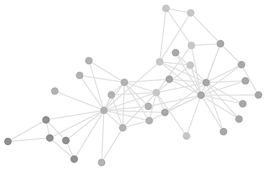
Graphs are a way to formally represent a network, or a collection of interconnected objects. They are really quite simple. They are a collection of nodes with edges connecting each node. Unlike something like a Tree, there are not very many rules for its structure at all. Nodes can be connected in any way. Even self-loops are allowed! Of course there does need to be at least one single node for a graph to be considered a graph.

Some graphs do however have certain attributes that influence its structure. The edges within graphs can be directional. A directed edge limits the direction in which that edge can be traveled. An undirected edge can be traversed in any direction. If all edge’s in a graph are directed then it is considered to be a digraph. And of course, if none of the edge’s are directed than it is considered an undirected graph. Simple enough, right?

So how are these graphs used in the context of Data Mining? There are many algorithms out there that can help us identify different characteristics of a graph. But deciding which algorithms will be the most valuable depends on what the graph represents. A common application of graph mining is social networks. Clustering algorithms are commonly used to help find groups of friends. You could represent web pages in a graph with each page being a node and all links to and from that page being edges. Clustering can be applied here as well and used for something like a page rank system. Other types of graphs such as a computer network may focus more on topology and estimating traffic. This is not far off from how the topic of this project, street networks, are analyzed.

Observing street networks alone can tell us many details about the surrounding urban environment. They can help us answer questions such as: Where are the most dense places in the city? Where are the most bottlenecks? How consistent are the orientation of streets? Analysis of existing street networks can help us plan for future urbanization projects.

DATA

So where is the data of these street networks coming from? All of the data is coming from Open Street Map (OSM). Launched in 2004, it is a collaborative project to create a free editable geographic database of the world. OSM is a go to source for all kinds of geospatial data around the world. It contains all sorts of data but of course we really are only interested in the street data. Thankfully, actually accessing the data has been made very easy by a Python package called OSMnx. OSMnx abstracts the entire process of accessing the OSM API’s and parsing the data in to graphs. It is built on top of NetworkX and GeoPandas libraries. OSMnx is developed and maintained by Geoff Boeing, the same researcher from the paper mentioned earlier. The package is specifically made for street network analysis.

METHODS

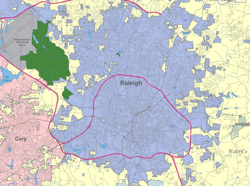
Graphs of street networks are modeled as intersections being nodes and all connecting streets being the edges. The three urban centers I’ll be exploring are Charlotte, Raleigh, and Greensboro since they are the most populated cities in North Carolina. As mentioned above, the process of loading these cities graphs is quite easy through OSMnx. I am able to load them from a geographic coordinate.

import networkx as nx
import osmnx as ox
import pandas as pd
import numpy as np
import matplotlib.pyplot as plt

#get charlotte street network from center point (longitude, latitude) 
Charlotte = [35.23284, -80.84857] 
Area = 6500 #meters from center
G_charlotte = ox.graph_from_point(center_point = Charlotte, dist=Area, network_type="drive", truncate_by_edge=True, clean_periphery=True)

I will not be evaluating the entire areas of the cities but rather a (somewhat arbitrarily) set distance from the center for each city.

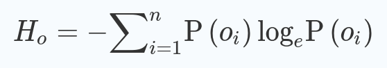
Once the graph is loaded into memory, we can start calculating some metrics. Once again, this whole process will be rather painless thanks to OSMnx. There are plenty of stats that can be calculated for these graphs but a few in particular stick out to me. The first of which is density. We can measure the density of nodes and edges in the graph by kilometer. Next, average Circuity seemed to be interesting. Circuity measures the curvature of streets by comparing the straight line distance to the length of edges between nodes. Lastly, and probably the most interesting stat, is Orientation Entropy. Orientation Entropy is calculated by first generating a bearing attribute for each intersection. Next, we want to group all the intersections by their bearing. In my case, I chose to group into 36 groups, one bin for every 10 degrees. Next we calculate entropy by summing the proportions of these groups times the natural logarithm of said proportion. And then negating the result so that it is positive.

#get basic stats
stats = ox.basic_stats(G_proj, area=graph_area_m, clean_int_tol=15)

# unpack dicts into individiual keys:values
for k, count in stats["streets_per_node_counts"].items():
    stats["{}way_int_count".format(k)] = count
for k, proportion in stats["streets_per_node_proportions"].items():
    stats["{}way_int_prop".format(k)] = proportion

# delete the no longer needed dict elements
del stats["streets_per_node_counts"]
del stats["streets_per_node_proportions"]

# load as a pandas dataframe
charlotte_stats = pd.DataFrame(pd.Series(stats, name="value")).round(3)

#get entropies
Gs = [G_charlotte, G_raleigh, G_greensboro]
GUs = []
cities = ['Charlotte', 'Raleigh', 'Greensboro']

for g in Gs:
    GUs.append(ox.add_edge_bearings(ox.get_undirected(g)))
    
entropies = []
for gu in GUs:
    entropies.append(ox.bearing.orientation_entropy(gu, num_bins = 36))

RESULTS

I created a dataframe containing the stats for each city.

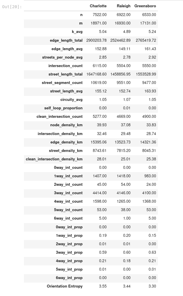
A few notable things caught my eye. First of all, Raleigh and Greensboro are much more similar to each other than to Charlotte. This is mainly seen in their densities. Charlotte is much more dense, meaning it has more streets and intersections than the others in the same amount of area. Charlotte also has a very high level of orientation entropy. We can really see this through a polar histogram that visualizes the bearing for each city.

Beyond density and orientation entropy, all three cities are actually pretty consistent with each other. This makes sense considering all of them are in the same region of North Carolina, I’d imagine geography influences development of cities.

Another cool figure I created visualizes edge betweeness centrality. This essentially measures the number of shortest paths that run through any given edge. We visualize this as a heat map of the graph.

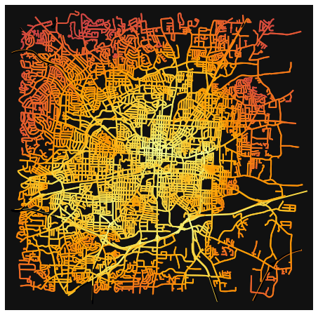
When looking at this graphs, we can see that Charlotte as a smaller concentration of the lighter edges in comparison to the others. It’s also interesting to see that Charlotte’s center grid is tilted about 45 degrees. I does not align North, South, East, and West like the other cities. I wonder if this contributes to its high entropy.

CONCLUSION

Coming into this project I had very little knowledge of graph analysis. I knew what a graph was but not much beyond that. After diving head first, I think I have learned a lot. I never realized how versatile graph analysis is. It can be applied to so many things. I’ve only scratched the surface with this project. None of this would have been possible without the OSMnx library. Being able to complete a meaningful analysis without a deep understanding of the underlying tools says a lot about the power of that library. Going forward, I certainly want to explore NetworkX and GeoPandas more. That being said, I am pretty pleased with the results of my project. I think I learned a lot of new things about these cities! I am starting to grow more interested in urban planning and seeing that there is a growing demand for urban informatics makes me think this would be something worth diving into further in the future.

I also want to reflect upon the course that this project is associated with this as a whole. Coming in, I really was a complete data science newbie. I had never dealt with Jupyter Notebooks, Pandas, or any type of Machine Learning. I had just a little experience with Python at least. Through the project based learning, I feel much more confident in all these tools moving forward. I aspire to be a data scientist and I truly believe everything I have learned in this course has been extremely valuable. I loved slowly building up my portfolio overtime and will continue to in the future as well. I wish more courses would follow this style of learning! It’s been a good semester!

CODE

You can find all the code associated with this post here.