Clustering Netflix Users

INTRODUCTION

Hello, again!

Today, I will be discussing a form of machine learning that I have not tackled before, that being Clustering. Clustering is much different from classification and regression because it is an unsupervised technique. Meaning that the data need not to be labeled. This has its pro’s and con’s. A pro is that data can be much larger since it does not need to be manually labeled. On the other hand, it is much more difficult to interpret results of the models. I’ll discuss clustering and the specific models to be implemented in more detail later.

I have chosen to try out the Netflix Prize data for this project. The origin of this data is actually very interesting. In 2006, Netflix held an open competition for the best collaborative filtering algorithm to predict user ratings of movies. The competition lasted nearly 4 years until a winner was finalized. The grand prize was $1,000,000. Netflix originally planned on holding a sequel but cancelled due to criticism over privacy concerns.

I will be treating the data a bit differently then what Netflix intended. The original competition was searching for a regression model however I will be implementing a clustering model instead. Both could theoretically be used in a recommendation system. This is essentially the question that I am trying to explore. Can customers be grouped based on their movie ratings? And how can said groupings be used in a recommendation system?

I will be discussing the data further soon, for now let’s dig into what clustering actually is.

WHAT IS CLUSTERING?

As stated before, clustering is an unsupervised machine learning technique. Data points are grouped in various ways depending on the specific clustering model being implemented. In theory, the data in each cluster should be similar in some way. The difficult part of clustering, and unsupervised learning in general, is that the resulting clusters cannot be easily interpreted. It’s hard to say if resulting clusters really have any value.

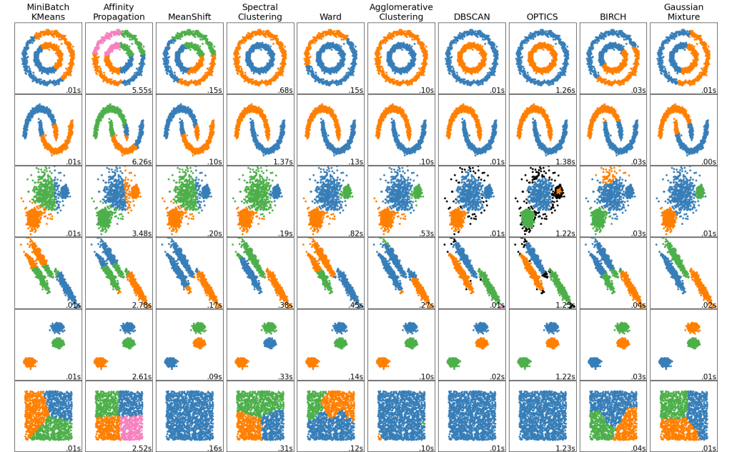
I’ll be implementing two models. K-Means clustering and Agglomerative Clustering. Both will achieve the same goal of creating clusters but differ in the methodologies of doing so.

K-Means creates clusters by first randomly placing K centroid points and then measures the euclidean distances of all other points to each centroid. Each point is grouped with the closest centroid which creates the clusters. The average point of each cluster is calculated and then is set as the new centroid. Then the process is repeated a set amount of times. K-Means is a very popular clustering algorithm since it is relatively easy to understand and is very fast (linear time complexity).

K-Means has a number of disadvantages such as the need to specify the number of clusters which is not always easily known. A common way to decide the number of clusters is simply by testing a range of cluster sizes and measuring the average variance of the clusters for each size and how much it changes as sizes increase. Also, due to the element of randomness in the algorithm, K-means models are not easily replicable.

Agglomerative clustering on the other hand is a hierarchical clustering model. Rather than starting with random centroid points like K-means does, agglomerative clustering starts by pairing points nearest to each other and iteratively pairs point or groups of points until a desired number of clusters is found.

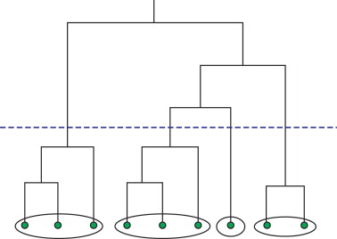
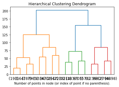
A key benefit of agglomerative clustering is that it is easy to visualize how groupings were made by using dendrogram.

A big disadvantage of hierarchical clustering is that it is rather slow (cubic time complexity), especially when compared to something like K-Means, thus making it not suitable for very large data.

DATA INTRODUCTION

Alright now that we have covered what clustering actually is, we can start to explore the details of the Netflix data.

I’ve heard of the competition in the past but have never really looked in to the specifics of the provided data. After a quick google search I was able to find a copy of the dataset on Kaggle. To my surprise, the dataset was quite large at over two gigabytes. It contains over 100 million ratings given by 480,189 customers to 17,770 movies. The data was separated into two main files, a “training_set” and a “movie_titles” files.

The movie titles data is already formatted as a CSV and contains columns for Movie ID, Year of Release, and Title. For my use case, I will not be utilizing the movie titles data since this is an unsupervised model. Although it does have value, say for looking up the centers of clusters.

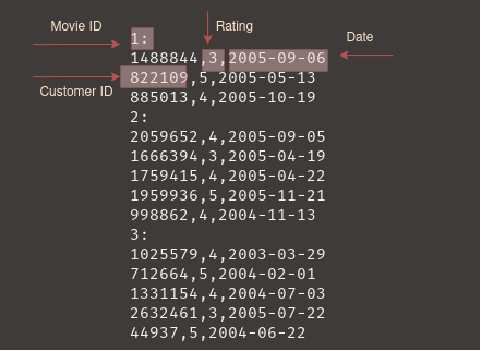
The training set is the most important in which contains all the ratings. It is formatted as a directory of 17,770 movies with each directory containing all the ratings for the movie. Luckily, the data has already been converted to a text file that is grouped by movie but still needs to be reformatted to follow convention for Pandas data frames.

DATA PROCESSING

The pre-processing of the data has easily been the most difficult part of the whole project. Not because the data is uncleaned but because of the raw size more than anything. Any type of operation that has to iterate over the entire data set almost always would kill my Jupyter Notebook kernel (due to memory limitations).

I tried exploring various solutions for my space limitations, such as using a cloud host and a lazy loading library. Unfortunately, a cloud host with sufficient resources would cost money and I don’t think that is worth it just for a single project. I did mess around quite a bit with Dask, a python library that integrates directly with Pandas and SciKit-Learn. It has a number of brilliant features but lazy loading is what I am interested in. Lazy loading would allow me to store dataframes on my disk rather than entirely in memory. Operations would be slower but a slightly longer wait would be worth it if it meant being able to keep all the data.

Dask is an amazing Python library but it is not super easy to use effectively. It takes a good amount of knowledge or parallel computing to be able to utilize and unfortunately it is a little out of my comfort zone at the moment. I was able to get some things working on Dask but I felt just learning the library itself was consuming too much time and the trade-off was not worth it. For the sake of completing this project in a timely manner, I’ve decided that some form of lossy compression may be necessary.

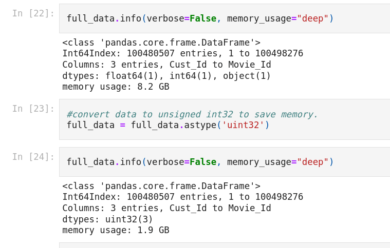
Moving forward, I did want to perform somewhat “methodical” data reduction and cleaning before resulting to randomly dropping rows. I was able to chug along by optimizing the data types and by utilizing NumPy and more efficient code.

The first order of business was to reformat the data so that it resembled a CSV file. To do this, I essentially just needed to remove all rows containing a movie ID and then create a column for Movie ID’s. The challenge was finding a way to make sure that each rating would correspond with the correct Movie ID. I was able to grab the index of each movie row since it contained the only null values in the dataset. Thankfully, the files was grouped by Movie ID so I could generate a correct Movie ID column just by iterating from 1 to 17770.

#get indices of Movie ID rows
movies = pd.DataFrame(pd.isnull(ratings.Rating))
movies = movies[movies['Rating'] == True]
movies = movies.reset_index()
movie_rows = np.array(movies['index'], dtype = np.int64)

#fast way to generate movie id column
new_rows = np.empty(len(ratings), dtype='int64')
temp = 0
for i, j in enumerate(movie_rows):
    if (i+1) == len(movie_rows):
        new_rows[j:len(ratings)] = (i+1)
    new_rows[temp:j] = i
    temp = j

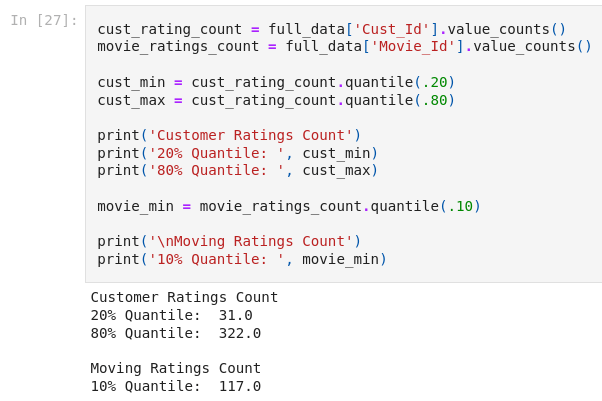
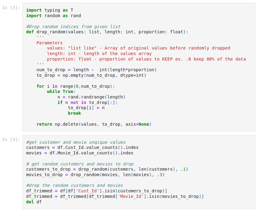
To further reduce the size, I removed outliers. Somehow, some users apparently rated nearly 17,000 movies which is almost the entire catalog. Not sure how that would be possible but I think it would throw off the model as that is not representative of normal user. I removed customers that had too many ratings and ones that had too little ratings. I decided to trim the top 20% and the bottom 20% of customers (in terms of rating count). A did a similar action for movies but only removed the bottom 10% in ratings received. I figured more ratings is a good thing for movies.

#perform drop
cust_low_threshold = list(cust_rating_count[cust_rating_count < cust_min].index)
cust_high_threshold = list(cust_rating_count[cust_rating_count > cust_max].index)
movies_to_drop = list(movie_ratings_count[movie_ratings_count < movie_min].index)
customers_to_drop = cust_low_threshold + cust_high_threshold
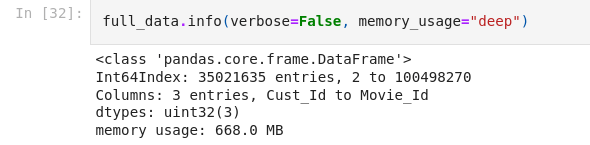
full_data = full_data[~full_data['Movie_Id'].isin(movies_to_drop)]
full_data = full_data[~full_data['Cust_Id'].isin(customers_to_drop)]

At this point, the data is formatted into three columns: Customer_Id, Rating, Movie_Id. The issue with this format is that the ID’s for both customers and movies are repeated throughout the data. I think it would better to reformat is with customer ID as the index and a column for each movie. Each cell will contain a rating if applicable, null otherwise. This process is similar to One-Hot Encoding.

The easiest way to perform this transformation is by using the Pandas pivot function. Unfortunately, this function is rather resource intensive and will still crash my kernel even with the cleaning done so far. At this point, randomly dropping customers and movies is the easiest option.

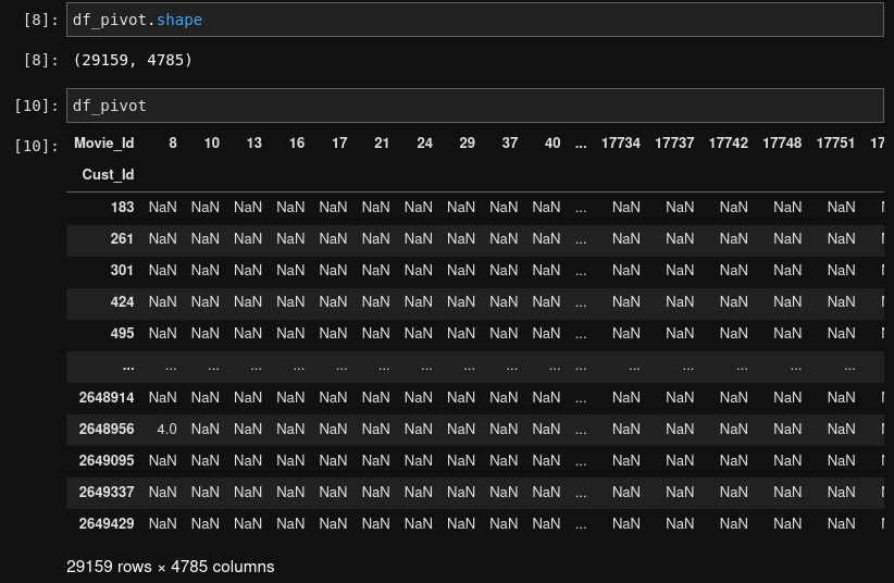
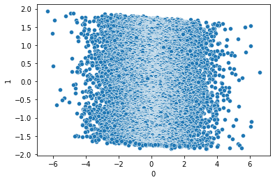
As you can see in the image above, that data is now nearly 5000 columns wide. While this isn’t necessarily a problem for the models, we won’t be able to visualize such high dimensional data. I will use Principal Component Analysis (PCA) to perform this dimensionality reduction.

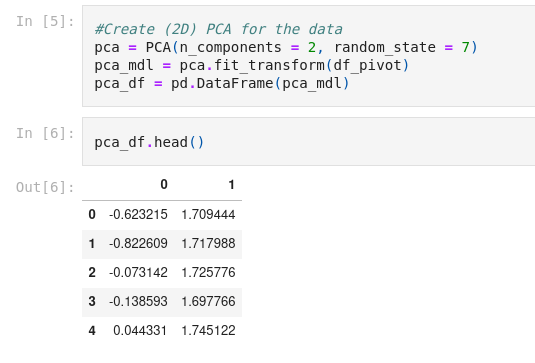
Alrighty! I think we are ready to move on to modeling the data.

MODELING

As stated before, I will be implementing both K-means and Agglomerative clustering.

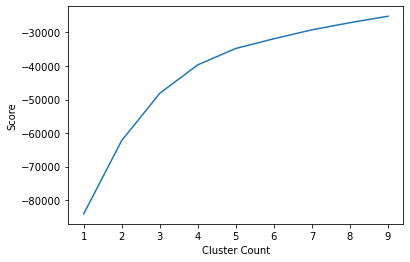
Starting with K-means, we first need to decide how many clusters to use. We’ll do this by creating an “elbow diagram” like the one shown earlier.

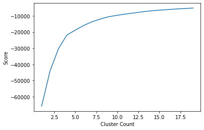
As you can see, around 4 or 5 clusters, the increase in score is negligible. We can now go ahead and visualize the clusters.

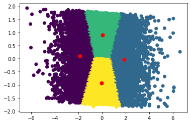
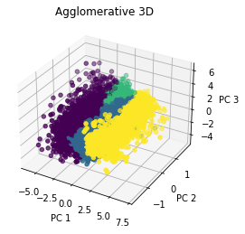
Now, for agglomerative clustering, I will also create 4 clusters.

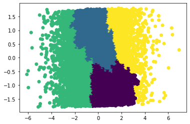
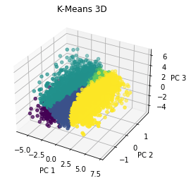
Interestingly, both models created somewhat similar clusters. Before jumping into analysis, I would like to also try a 3D PCA and run some models on that as well.

ANALYSIS

Coming in to this project, I imagined using clustering as a sort of recommendation system. I imagined using the clusters to implement collaborative filtering. However, it’s hard to say how effective this would be in practice and I think it is beyond the scope of this project to try testing a recommendation system. Based on our “elbow” diagram, it seemed that 4 clusters was optimal, and that seems to be a very small number if it were to be utilized in a recommendation system. I do think there are other applications that these clusters could be used for such as personalized advertisements (but of course Netflix does not run ads at the moment, but a company like Hulu which as a free subscription with ads could use a similar model). All and all, this is the biggest challenge of clustering. Interpreting the model and its clusters is no easy task. I did find it interesting that the shape of the clusters was relatively consistent across both types of models. I am not sure but I do believe that consistency across models may indicate that there are indeed some distinct valuable clusters.

I learned a lot from this project! Once again, pre-processing was essential for the modeling step. I think clustering has been the most challenging machine learning technique that I have dealt with so far. The black box nature of it makes it very difficult to interpret. However, the added challenge does make things a bit more fun.

CODE

Here is my code!